Quick start¶

sympde allows you to create symbolic expressions using differential/algebraic operators. It can be used to define strong or weak forms, when dealing with finite elements methods.

Strong forms¶

Assume you want to create the symbolic expression that is equivalent to

$\mathcal{L} u := - \nabla^2 u + u$

where $u$ denotes the unknown of 2 variables (2D).

In sympde, you can declare $u$ using

from sympde import Unknown

u = Unknown('u', ldim=2)

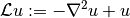
The expression associated to the operator $\mathcal{L}$ is then defined as

from sympde import grad, div

expr = - div(grad(u)) + u

you can also use a lambda expression

from sympde import grad, div

L = lambda u: - div(grad(u)) + u

As any sympy expression, you can take a look at the diagram of the expression tree:

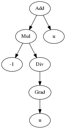
Expression tree for the 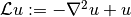$\mathcal{L} u := - \nabla^2 u + u$ operator.

Note

The above diagram was made using Graphviz and the dotprint function.

sympde allows to write more complicated expressions and it knows many differential calculus rules to perform the computation on its own.

Let us consider the following mathematical expression

$\partial_x \partial_y uv$

The symbolic associated expression can be achieved using

from sympde import Unknown
from sympde import dx, dy

u = Unknown('u', ldim=2)
v = Unknown('v', ldim=2)

expr = dx(dy(u*v))

Since we are using the atomic operators dx and dy, the expression will be automatically evaluated, in opposition to the use of grad or div. Hence, result is

>>>  u*dx(dy(v)) + v*dx(dy(u)) + dx(u)*dy(v) + dx(v)*dy(u)

and the associated expression tree is

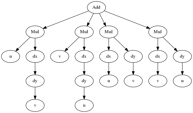
Expression tree for $\partial_x \partial_y uv$ .

When evaluated, sympde differential operators are linear operators. Which means that the following code:

from sympde import Unknown
from sympde import dx, dy

u = Unknown('u', ldim=2)
v = Unknown('v', ldim=2)

expr = dy(2*u+3*v)

will return:

>>> 2*dy(u) + 3*dy(v)

sympde introduces the notion of a constant through the class Constant. As expected, applying a differential operator on it will return 0:

from sympde import Unknown, Constant
from sympde import dx

u = Unknown('u', ldim=1)
alpha = Constant('alpha')

expr = dx(alpha*u) + dx(dx(2*u))

The result is:

>>> alpha*dx(u) + 2*dx(dx(u))

You can also apply a differential operator on an analytical function, which is useful to compute solution/rhs of a partial differential equation:

from sympde import Constant
from sympde import dx, dy
from sympy.abc import x, y
from sympy import cos, exp

alpha = Constant('alpha')

L = lambda u: -dx(dx(u)) - dy(dy(u)) + alpha * u

expr = L(cos(y)*exp(-x**2))

The result is:

>>> alpha*exp(-x**2)*cos(y) - 4*x**2*exp(-x**2)*cos(y) + 3*exp(-x**2)*cos(y)

sympy undefined can also be used:

from sympde import Constant
from sympde import dx, dy
from sympy.abc import x, y
from sympy import Function

alpha = Constant('alpha')
f = Function('f')

L = lambda u: -dx(dx(u)) - dy(dy(u)) + alpha * u

expr = L(f(x,y))

which gives:

>>> alpha*f(x, y) - Derivative(f(x, y), x, x) - Derivative(f(x, y), y, y)

Weak forms¶

Other useful notions for partial differential equations are bilinear/linear forms, which are needed when using variational methods such as finite elements.

Variational forms come with two very important concepts:

FunctionSpace: mathematical function space. It can be a Sobolev space for example.
TestFunction: a member of FunctionSpace

Bilinear form¶

Unlike fenics, sympde does not distinguish between test and trial functions; there is no type for trial functions. In fact, they are implicitly infered from the arguments of a bilinear form. The later is defined like a sympy Lambda object. This means that the user must provide:

a couple describing test and trial functions
a symbolic expression of the bilinear form

The nice thing about this approach is that it allows calling the bilinear form with different arguments and then ensures more modularity and reuse of the abstract mathematical models.

The following example shows how to define the weak formulation of the Laplace operator

from sympde import grad, dot
from sympde import FunctionSpace
from sympde import TestFunction
from sympde import BilinearForm

V = FunctionSpace('V', ldim=2)
U = FunctionSpace('U', ldim=2)

v = TestFunction(V, name='v')
u = TestFunction(U, name='u')

a = BilinearForm((v,u), dot(grad(v), grad(u)) + v*u)

Let’s take a look at the expression tree:

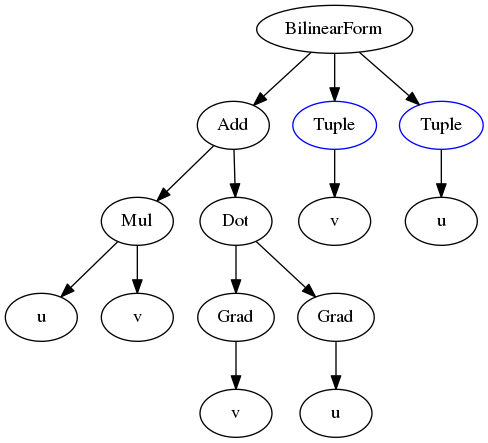
Expression tree for Laplace weak form.

We notice that the BilinearForm arguments are presented as a Tuple. The reason is that you can also define a bilinear form that is associated to a system of expressions.

As any sympde expression, a BilinearForm can be printed, calling

print(a)

would give

>>> u*v + Dot(Grad(v), Grad(u))

The following example implements a 1D wave model:

from sympde import dx
from sympde import FunctionSpace
from sympde import TestFunction
from sympde import BilinearForm

V = FunctionSpace('V', ldim=1)
W = FunctionSpace('W', ldim=1)

T = Constant('T', real=True, label='Tension applied to the string')
rho = Constant('rho', real=True, label='mass density')
dt = Constant('dt', real=True, label='time step')

# trial functions
u = TestFunction(V, name='u')
f = TestFunction(W, name='f')

# test functions
v = TestFunction(V, name='v')
w = TestFunction(W, name='w')

mass = BilinearForm((v,u), v*u)
adv  = BilinearForm((v,u), dx(v)*u)

expr = rho*mass(v,u) + dt*adv(v, f) + dt*adv(w,u) + mass(w,f)
a = BilinearForm(((v,w), (u,f)), expr)

Todo

add example using Mapping

Todo

add example using vector test functions

Todo

add example using Field

Linear form¶

Linear forms are more simple to create, but follow the same logic:

from sympde import FunctionSpace
from sympde import TestFunction
from sympde import LinearForm
from sympy import cos

V = FunctionSpace('V', ldim=2)

v = TestFunction(V, name='v')

x,y = V.coordinates

b = LinearForm(v, cos(x-y)*v)

Notice that the space gives access to the coordinates, which can be used for callable functions, such as the cos in our example.

Function form¶

A FunctionForm allows you to write expressions that can be integrated over the compputational domain. It can be defined as follows:

from sympde import grad, div
from sympde import FunctionSpace
from sympde import Field
from sympde import FunctionForm
from sympy import cos, pi

V = FunctionSpace('V', ldim=1)
F = Field('F', space=V)

x = V.coordinates

b = FunctionForm(div(grad(F-cos(2*pi*x))))

Evaluation¶

The purpose of sympde is to declare objects that are needed to write an abstract mathematical model for problems involving partial differential equations. It does not provide any discretization. However, it provides you also with algorithms to manipulate the symbolic expressions. For example, when using generic operators such as grad or div, the expression is not evaluated. For this reason, sympde provides the function evaluate that allows you to transform your expression into atomic operators such as dx, dy, dz. In the following example, we evaluate the Laplace operator:

from sympde import grad, dot
from sympde import FunctionSpace
from sympde import TestFunction
from sympde import BilinearForm
from sympde import evaluate

V = FunctionSpace('V', ldim=2)
U = FunctionSpace('U', ldim=2)

v = TestFunction(V, name='v')
u = TestFunction(U, name='u')

a = BilinearForm((v,u), dot(grad(v), grad(u)) + v*u)
print(evaluate(a))

The result is the following expression:

>>> u_x*v_x + u_y*v_y + u*v

You can then use this expression inside your code generation module to define the weak form associated to the bilinear form. What sympde does is the following:

converts generic operators such as grad or div to their atomic expressions
converts an atomic expression like dx(u) to u_x which can be used directly inside your python code (kernel of finite elements for example)

If you only want to convert the generic operators into atomic operators, then you may use the atomize function:

from sympde import grad, dot
from sympde import FunctionSpace
from sympde import TestFunction
from sympde import BilinearForm
from sympde import atomize

V = FunctionSpace('V', ldim=2)
U = FunctionSpace('U', ldim=2)

v = TestFunction(V, name='v')
u = TestFunction(U, name='u')

a = BilinearForm((v,u), dot(grad(v), grad(u)) + v*u)
print(atomize(a.expr))

The result is then:

>>> u*v + dx(u)*dx(v) + dy(u)*dy(v)

Notice that atomize is a low level function and is called inside evaluate. For this reason, atomize only operates on the expression of sympde forms.

Printing¶

Latex¶

A symbolic expression can be printed in latex. This is done by calling the function latex on your expression or sympde forms.

from sympde import grad, div
from sympde import Unknown
from sympde.printing import latex

u = Unknown('u', ldim=2)

print(latex(- div(grad(u)) + u))

which gives the following result:

>>> u - \nabla \cdot \nabla{u}

$u - \nabla \cdot \nabla{u}$

A BilinearForm can also be printed:

from sympde import grad, dot
from sympde import FunctionSpace
from sympde import TestFunction
from sympde import BilinearForm
from sympde import atomize
from sympde.printing import latex

V = FunctionSpace('V', ldim=2)
U = FunctionSpace('U', ldim=2)

v = TestFunction(V, name='v')
u = TestFunction(U, name='u')

a = BilinearForm((v,u), dot(grad(v), grad(u)) + v*u)
print(latex(a))

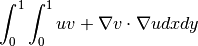
which returns

>>> \int_{0}^{1}\int_{0}^{1} u v + \nabla{v} \cdot \nabla{u} dxdy

$\int_{0}^{1}\int_{0}^{1} u v + \nabla{v} \cdot \nabla{u} dxdy$

Quick start¶

Strong forms¶

Weak forms¶

Bilinear form¶

Linear form¶

Function form¶

Evaluation¶

Printing¶

Latex¶

sympde

Navigation

Related Topics